Fully worked-out analysis using a Bayesian regression with brms

library(tidyverse)
theme_set(theme_minimal())
library(ggrepel)
library(learnB4SS)
library(extraDistr)
library(HDInterval)
library(tidybayes)
library(bayesplot)
library(modelr)
library(broom.mixed)
library(brms)

data("incomplete")

# Set custom b4ss colours
b4ss_colors <- c(purple = "#8970FF", orange = "#FFA70B")
scale_fill_b4ss <- function(...) {
  scale_fill_manual(..., values = c(b4ss_colors[[1]], b4ss_colors[[2]]))
}
scale_color_b4ss <- function(...) {
  scale_color_manual(..., values = c(b4ss_colors[[1]], b4ss_colors[[2]]))
}

Study overview and data

glimpse(incomplete)
#> Rows: 6,144
#> Columns: 8
#> $ order           <dbl> 9, 10, 11, 12, 13, 14, 15, 16, 17, 18, 19, 20, 21, 22,…
#> $ speaker_voice   <chr> "VP11", "VP10", "VP07", "VP15", "VP06", "VP09", "VP08"…
#> $ item_pair       <dbl> 19, 11, 14, 23, 7, 15, 3, 13, 24, 2, 5, 20, 3, 8, 4, 9…
#> $ RT              <dbl> 1531, 1009, 633, 1852, 3606, 4493, 15186, 1995, 940, 4…
#> $ correct         <dbl> 1, 1, 1, 1, 0, 1, 0, 0, 0, 0, 0, 0, 1, 1, 0, 1, 1, 1, …
#> $ correct_voicing <chr> "voiceless", "voiceless", "voiced", "voiced", "voicele…
#> $ listener        <chr> "L01", "L01", "L01", "L01", "L01", "L01", "L01", "L01"…
#> $ repetitiontype  <chr> "first", "first", "first", "first", "first", "first", …

Model formula

m1_bf <- brmsformula(
  correct ~
    correct_voicing *
    repetitiontype +
    # random slopes for interaction across listeners
    (correct_voicing * repetitiontype | listener) +
    # random slopes for interaction across speaker voices
    (correct_voicing * repetitiontype | speaker_voice) +
    # random slopes for interaction across minimal pairs
    (correct_voicing * repetitiontype | item_pair),
  family = bernoulli()
)

Priors and prior predictive checks

Prior distribution of the outcome variable (likelihood, family)

\[correct_i \sim Bernoulli(p)\]

y <- dbern(c(0, 1), p = 0.75)

ggplot() +
  aes(c("0", "1"), y) +
  geom_linerange(aes(ymin = 0, ymax = y), size = 2, colour = b4ss_colors) +
  geom_point(size = 5, colour = b4ss_colors) +
  ylim(0, 1) +
  labs(x = "outcome", y = "p")
#> Warning: Using `size` aesthetic for lines was deprecated in ggplot2 3.4.0.
#> ℹ Please use `linewidth` instead.
#> This warning is displayed once every 8 hours.
#> Call `lifecycle::last_lifecycle_warnings()` to see where this warning was
#> generated.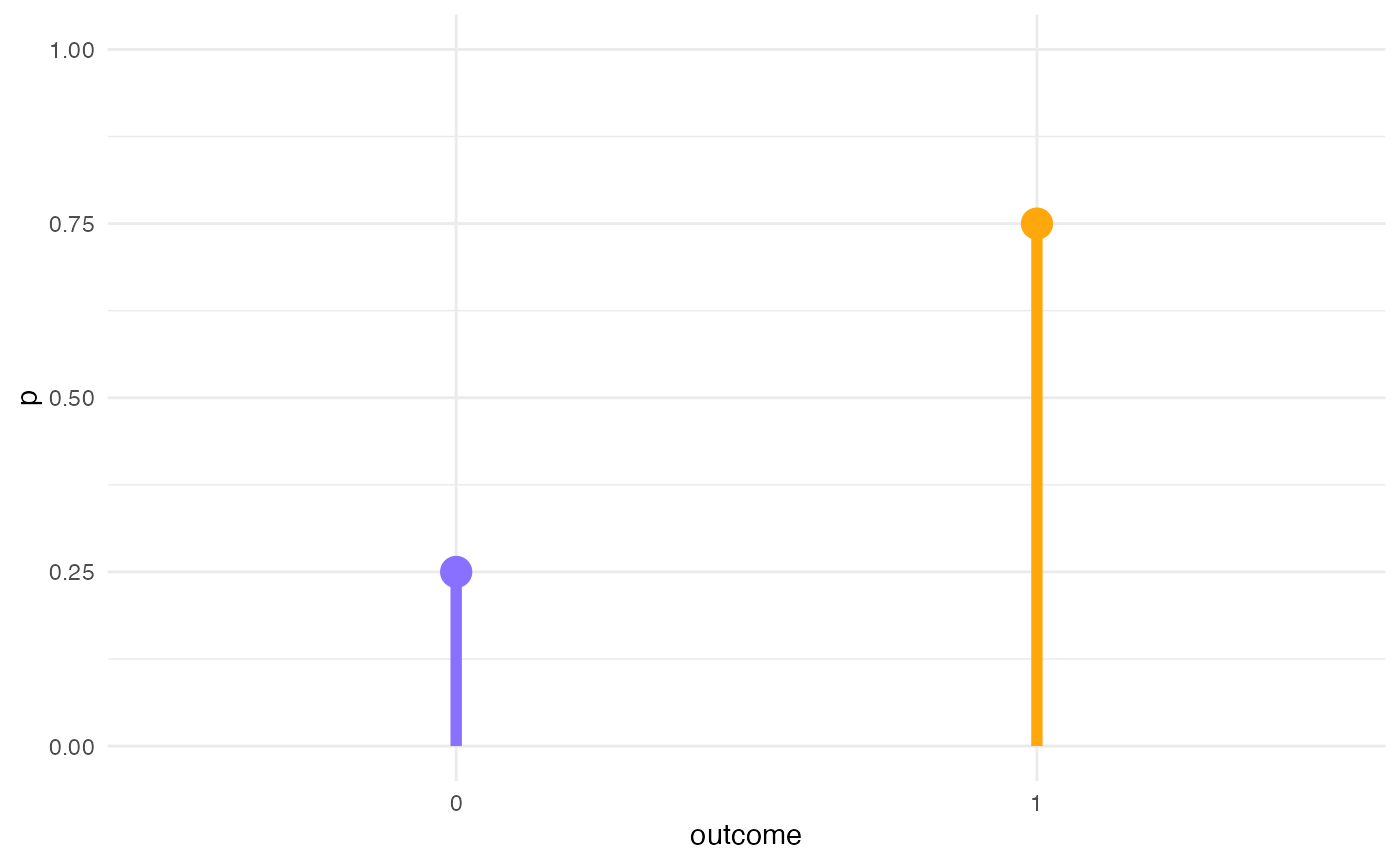

Get priors

# get_prior(m1_bf, data = incomplete)
get_prior(m1_bf, data = incomplete) %>%
  as_tibble() %>%
  select(prior:group)
#> # A tibble: 25 × 4
#>    prior                  class     coef                                   group
#>    <chr>                  <chr>     <chr>                                  <chr>
#>  1 ""                     b         ""                                     ""   
#>  2 ""                     b         "correct_voicingvoiceless"             ""   
#>  3 ""                     b         "correct_voicingvoiceless:repetitiont… ""   
#>  4 ""                     b         "repetitiontyperepeated"               ""   
#>  5 "lkj(1)"               cor       ""                                     ""   
#>  6 ""                     cor       ""                                     "ite…
#>  7 ""                     cor       ""                                     "lis…
#>  8 ""                     cor       ""                                     "spe…
#>  9 "student_t(3, 0, 2.5)" Intercept ""                                     ""   
#> 10 "student_t(3, 0, 2.5)" sd        ""                                     ""   
#> # ℹ 15 more rows

Log-odds space

dots <- tibble(
  p = seq(0.1, 0.9, by = 0.1),
  log_odds = qlogis(p)
)

tibble(
  p = seq(0, 1, by = 0.001),
  log_odds = qlogis(p)
) %>%
  ggplot(aes(p, log_odds)) +
  geom_hline(yintercept = 0, alpha = 0.5) +
  geom_vline(xintercept = 0.5, linetype = "dashed") +
  geom_line(size = 2, colour = b4ss_colors[2]) +
  geom_point(data = dots, size = 4, colour = b4ss_colors[1]) +
  scale_x_continuous(breaks = seq(0, 1, by = 0.1), minor_breaks = NULL) +
  scale_y_continuous(breaks = seq(-6, 6, by = 2), minor_breaks = NULL) +
  labs(
    title = "Correspondence between probabilities and log-odds",
    x = "probability",
    y = "log-odds"
  )

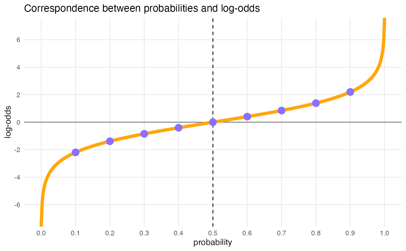
# log-odds = 0; get probability
glue::glue("Log-odds 0 = p(", plogis(0), ")")
#> Log-odds 0 = p(0.5)
# p = 0.5; get log-odds
glue::glue("p(0.5) = log-odds ", qlogis(0.5))
#> p(0.5) = log-odds 0

cat("\n\n")

# log-odds = 1.5; get probability
glue::glue("Log-odds 1.5 = p(", round(plogis(1.5), 4), ")")
#> Log-odds 1.5 = p(0.8176)
# p = 0.5; get log-odds
glue::glue("p(0.8176) = log-odds ", round(qlogis(0.8175745), 4))
#> p(0.8176) = log-odds 1.5

Prior for the intercept

# Log-odds to p
plogis(-6) # ~= 0 
#> [1] 0.002472623
plogis(6) # ~= 1
#> [1] 0.9975274

x <- seq(-15, 15, by = 0.1)
# 95% Cri [-6, +6] => SD = 6/2 = 3
y <- dnorm(x, mean = 0, sd = 3)

ggplot() +
  aes(x, y) +
  geom_line(size = 1.5, colour = b4ss_colors[1]) +
  labs(x = "log-odds")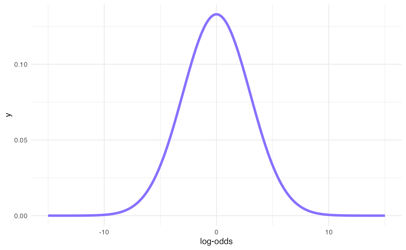

Prior for b

# Log-odds to odds
exp(-2) # ~= 0
#> [1] 0.1353353
exp(2) # ~= 7
#> [1] 7.389056

x <- seq(-4, 4, by = 0.1)
# 95% Cri [-2, +2] => SD = 2/2 = 1
y <- dnorm(x, mean = 0, sd = 1)

ggplot() +
  aes(x, y) +
  geom_line(size = 1.5, colour = b4ss_colors[1]) +
  labs(x = "log-odds")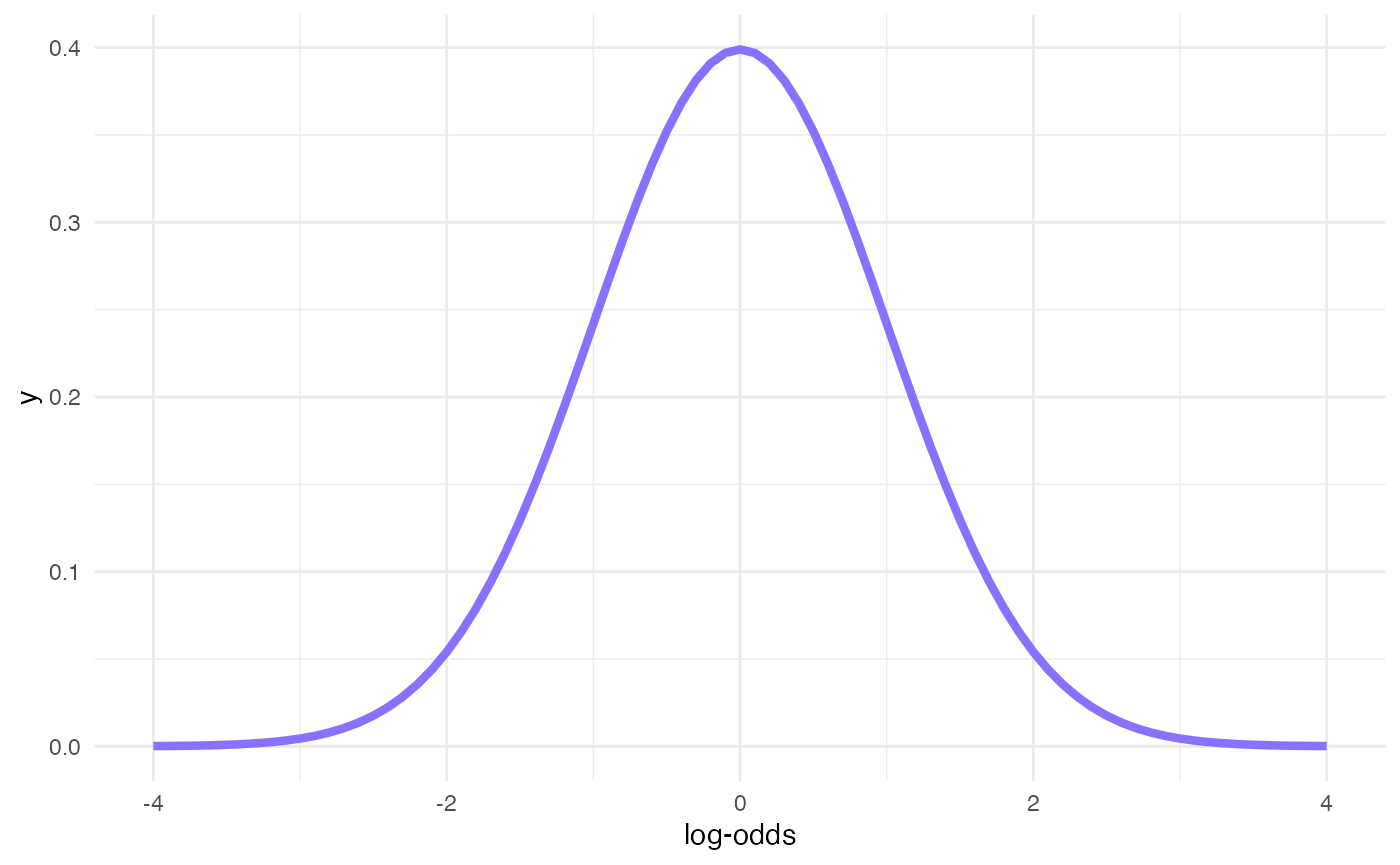

Prior for sd

inverseCDF(c(0.025, 0.975), phcauchy, sigma = 0.1)
#> [1] 0.003930135 2.545175934

x <- seq(0, 3, by = 0.01)
y <- dhcauchy(x, sigma = 0.1)

ggplot() +
  aes(x, y) +
  geom_line(size = 1, colour = b4ss_colors[2]) +
  labs(x = "log-odds")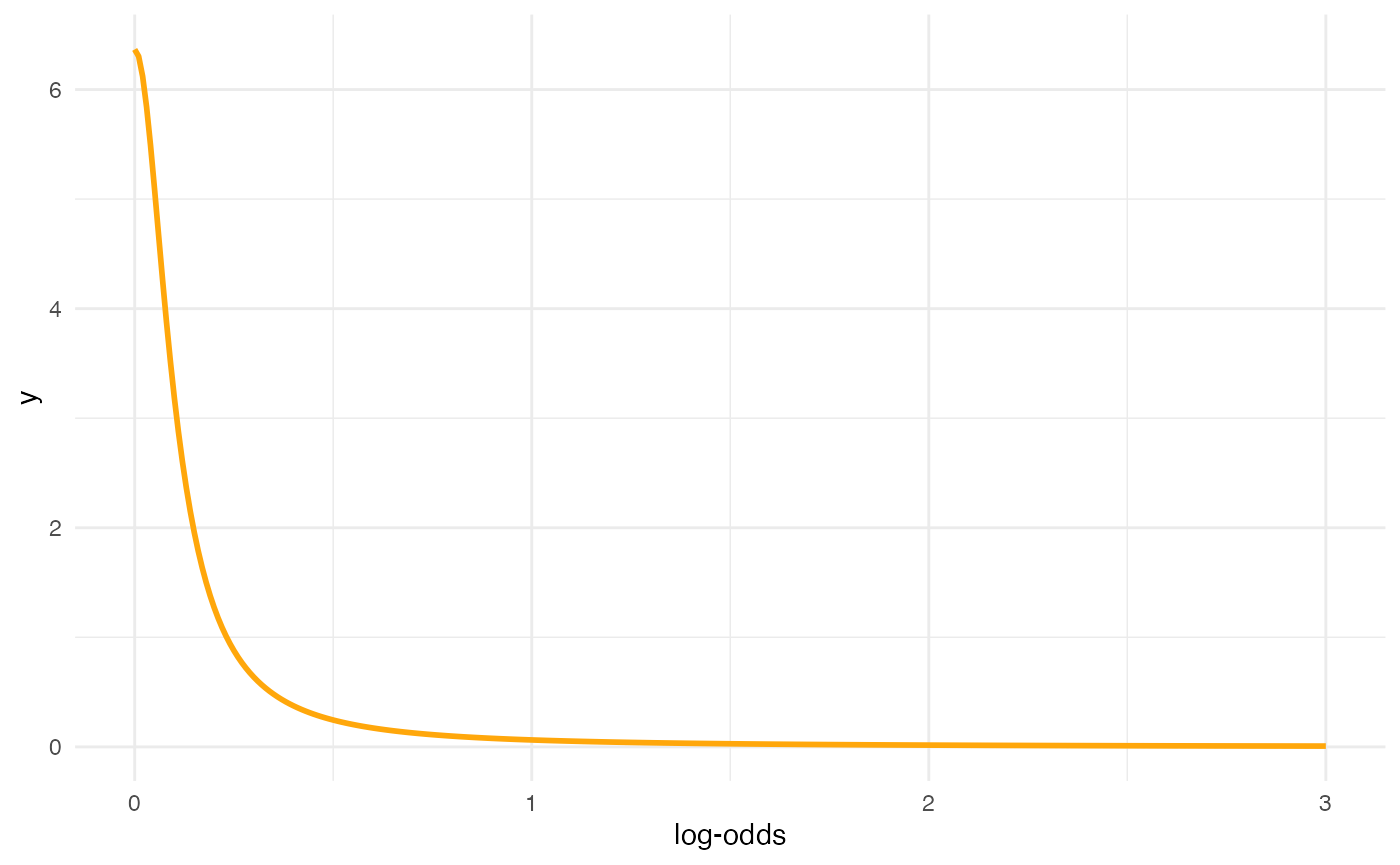

Set priors

priors <- c(
  prior(normal(0, 3), class = Intercept),
  prior(normal(0, 1), class = b),
  prior(cauchy(0, 0.1), class = sd),
  prior(lkj(2), class = cor)
)

Prior predictive checks

m1_priorpc <- brm(
  m1_bf,
  data = incomplete,
  prior = priors,
  sample_prior = "only",
  file = system.file("extdata/m1_priorpc.rds", package = "learnB4SS")
)

conditional_effects(m1_priorpc, effects = "correct_voicing:repetitiontype")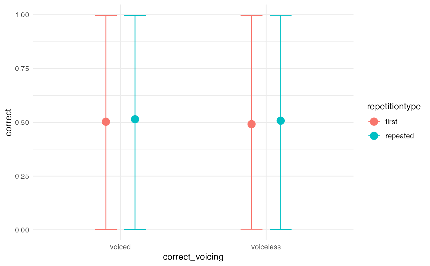

Let’s try VERY strong priors for comparison

priors_strong <- c(
  prior(normal(2, 0.1), class = Intercept),
  prior(normal(1, 0.1), class = b),
  prior(cauchy(0, 0.1), class = sd),
  prior(lkj(2), class = cor)
)

m1_priorpc_strong <- brm(
  m1_bf,
  data = incomplete,
  prior = priors_strong,
  sample_prior = "only",
  cores = 4,
  file = system.file("extdata/m1_priorpc_strong.rds", package = "learnB4SS")
)

conditional_effects(m1_priorpc_strong, effects = "correct_voicing:repetitiontype")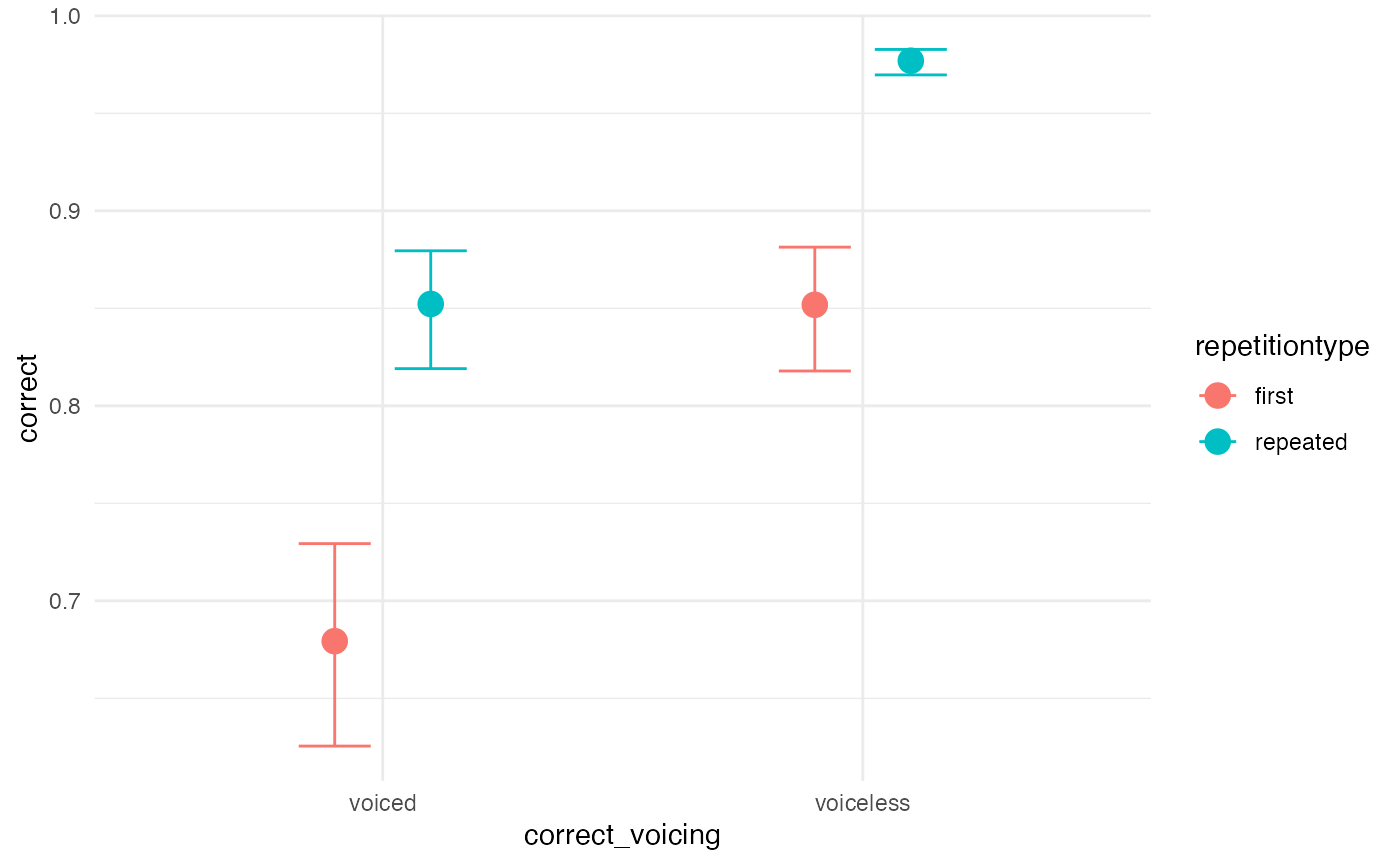

Run model

m1_full <- brm(
  m1_bf,
  data = incomplete,
  prior = priors,
  cores = parallel::detectCores(), 
  chains = 4, 
  iter = 2000, 
  warmup = 1000, 
  file = system.file("extdata/m1_full.rds", package = "learnB4SS")
)

Model output and interpretation

Checks and diagnostics

# Sample data from the generative model and compare with real data
pp_check(m1_full, nsamples = 200)
#> Warning: Argument 'nsamples' is deprecated. Please use argument 'ndraws'
#> instead.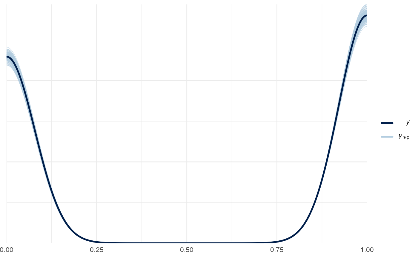

# Generate trace and density plots for MCMC samples
# Only looking at pop-level parameters (no SDs or cor)
plot(m1_full, pars = "^b_")
#> Warning: Argument 'pars' is deprecated. Please use 'variable' instead.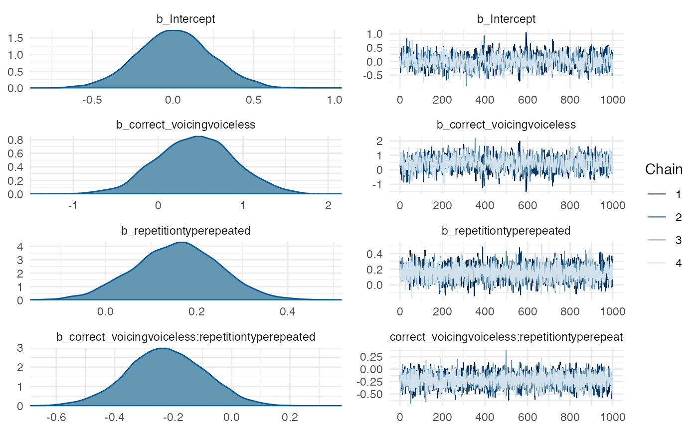

# Pairs plots to help spot degeneracies (doesn't apply here but 
# useful if you have divergent transitions)
pairs(m1_full, pars = "^b_")
#> Warning: Argument 'pars' is deprecated. Please use 'variable' instead.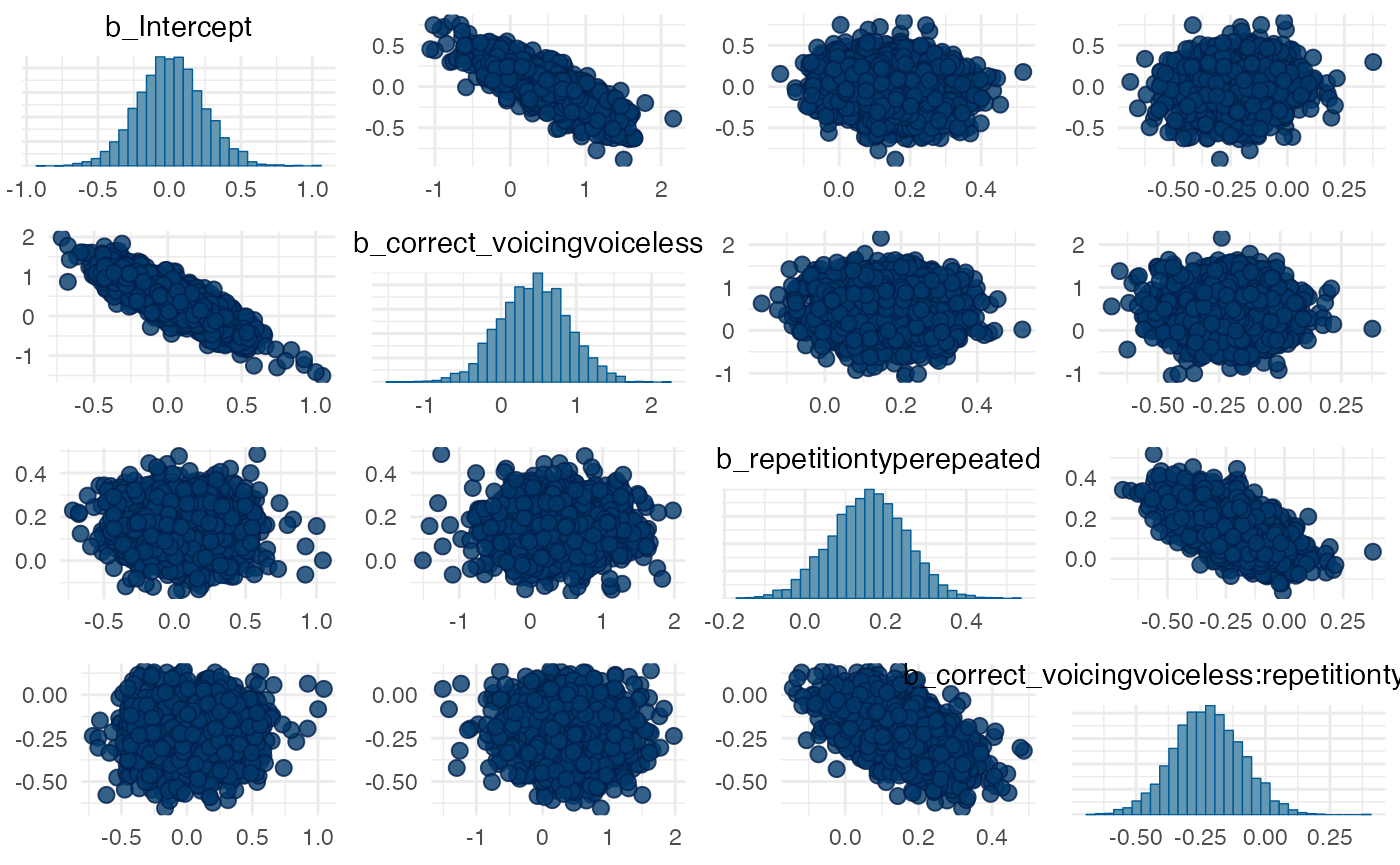

# Check Rhat and ESS (remove the rest of the output so it doesn't distract)
summary(m1_full)$fixed[, 5:7]
#>                                                      Rhat  Bulk_ESS Tail_ESS
#> Intercept                                       1.0049420  977.8247 1358.471
#> correct_voicingvoiceless                        1.0045544 1226.8754 1982.232
#> repetitiontyperepeated                          1.0013897 3884.5014 2915.458
#> correct_voicingvoiceless:repetitiontyperepeated 0.9999374 4262.5928 2502.050

Prior sensitivity analysis

m1_fixed <- tidy(m1_full, effects = "fixed", conf.level = 0.95, fix.intercept = FALSE) %>%
  mutate(
    ci_width = abs(conf.low - conf.high)
  )
#> Warning in tidy.brmsfit(m1_full, effects = "fixed", conf.level = 0.95,
#> fix.intercept = FALSE): some parameter names contain underscores: term naming
#> may be unreliable!
m1_fixed
#> # A tibble: 4 × 8
#>   effect component term           estimate std.error conf.low conf.high ci_width
#>   <chr>  <chr>     <chr>             <dbl>     <dbl>    <dbl>     <dbl>    <dbl>
#> 1 fixed  cond      Intercept        0.0125    0.231   -0.437     0.477     0.914
#> 2 fixed  cond      correct_voici…   0.439     0.461   -0.454     1.33      1.79 
#> 3 fixed  cond      repetitiontyp…   0.156     0.0938  -0.0272    0.336     0.363
#> 4 fixed  cond      correct_voici…  -0.224     0.133   -0.486     0.0319    0.518

m1_fixed %>%
  mutate(
    theta = c(0, 0, 0, 0),
    sigma_prior = c(3, 1, 1, 1),
    z = abs((estimate - theta) / std.error), # it's called here std.error but is the standard deviation
    s = 1 - (std.error^2 / sigma_prior^2)
  ) %>%
  ggplot(aes(s, z, label = term)) +
  geom_point() +
  geom_label_repel(arrow = arrow()) +
  xlim(0, 1) + ylim(0, 5)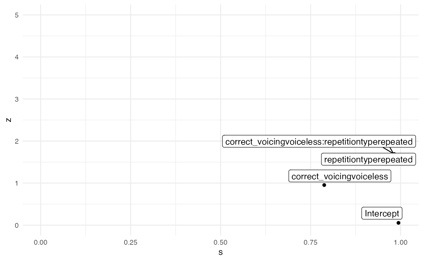

labels <- tibble(
  x = c(0.25, 0.25, 0.6, 0.75),
  y = c(1.25, 3.75, 1.25, 3.75),
  labs = c("Poorly identified", "Prior/Posterior\nconflict", "Ideal", "Overfit")
)

m1_fixed %>%
  mutate(
    theta = c(0, 0, 0, 0),
    sigma_prior = c(3, 1, 1, 1),
    z = abs((estimate - theta) / std.error), # it's called here std.error but is the standard deviation
    s = 1 - (std.error^2 / sigma_prior^2)
  ) %>%
  ggplot(aes(s, z, label = term)) +
  annotate("rect", xmin = 0, ymin = 0, xmax = 0.5, ymax = 2.5, alpha = 0.5, fill = "#e66101") +
  annotate("rect", xmin = 0, ymin = 2.5, xmax = 0.5, ymax = 5, alpha = 0.5, fill = "#fdb863") +
  annotate("rect", xmin = 0.5, ymin = 0, xmax = 1, ymax = 2.5, alpha = 0.5, fill = "#b2abd2") +
  annotate("rect", xmin = 0.5, ymin = 2.5, xmax = 1, ymax = 5, alpha = 0.5, fill = "#5e3c99") +
  geom_label(data = labels, aes(x, y, label = labs), colour = "white", fill = "black") +
  geom_label_repel(fill = NA) +
  geom_point() +
  xlim(0, 1) + ylim(0, 5)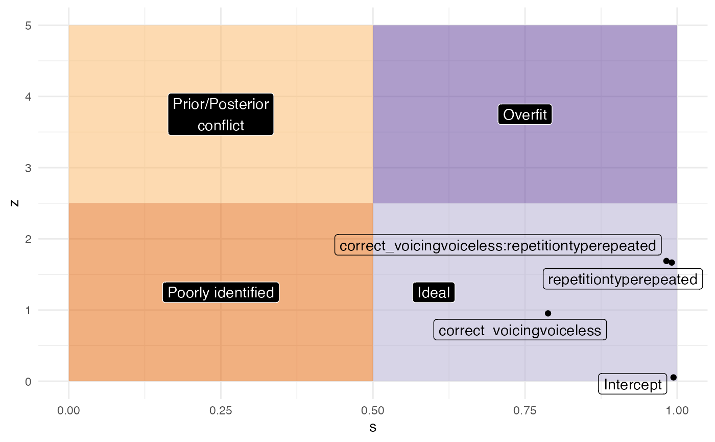

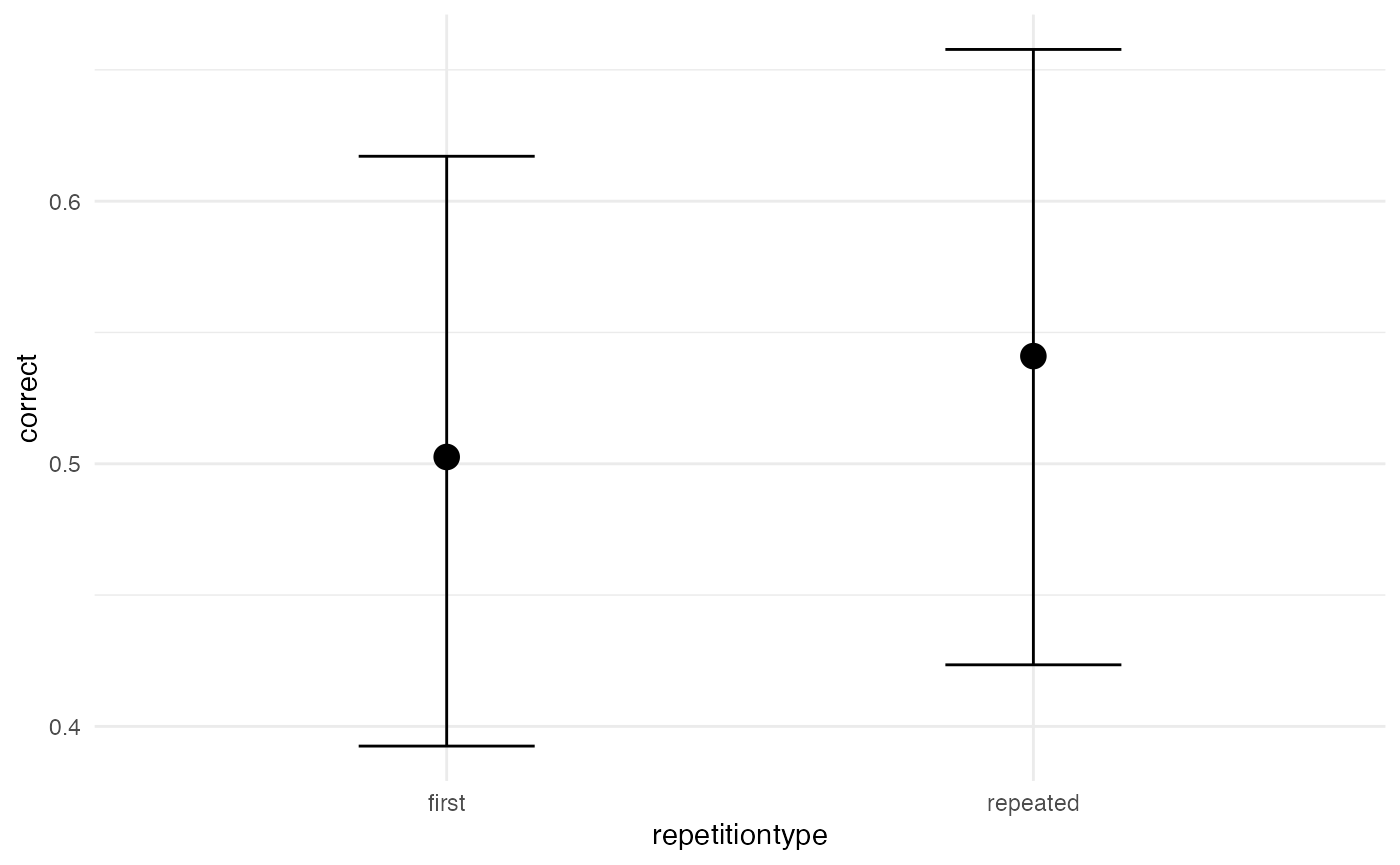
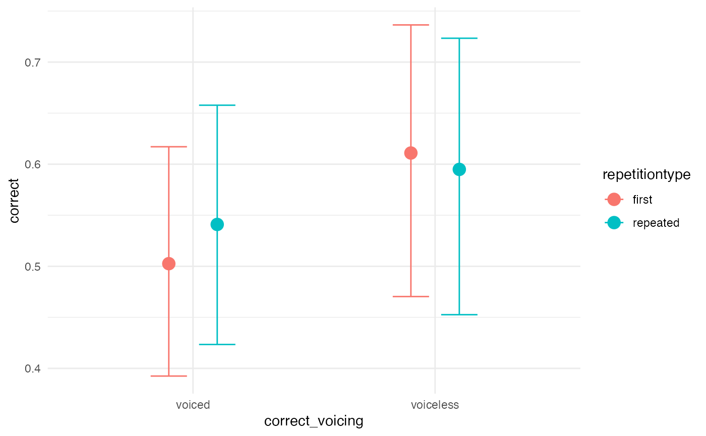
Visual effects

A quick and dirty way to assess the posterior predictions is using the conditional_effects() function. It is also useful because it plots the data into the original scale.

# quick and dirty plot on the original scale
plot(conditional_effects(m1_full), ask = FALSE)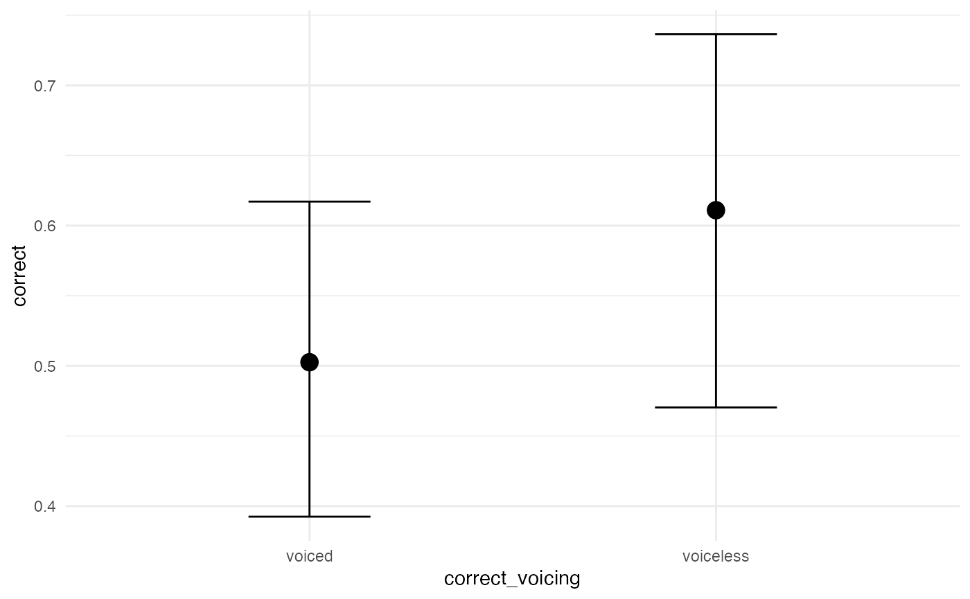

We can also plot the posterior distributions of our population-level coefficients. This can be conveniently done with the bayesplot package.

posterior <- as.matrix(m1_full)

mcmc_areas(posterior,
           pars = c("b_Intercept", 
                    "b_correct_voicingvoiceless", 
                    "b_repetitiontyperepeated", 
                    "b_correct_voicingvoiceless:repetitiontyperepeated"),
           # arbitrary threshold for shading probability mass
           prob = 0.83)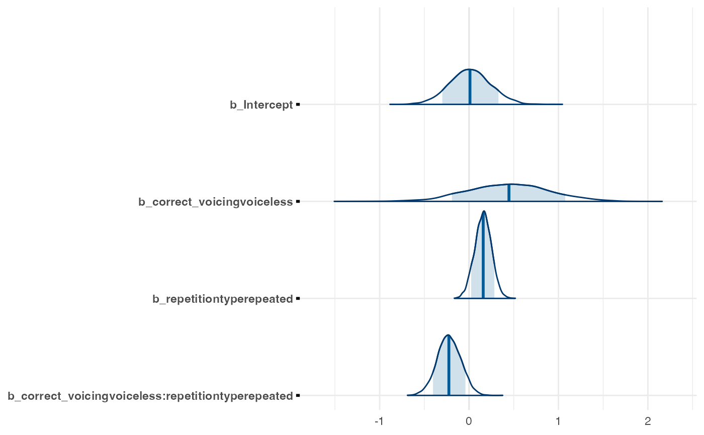 

For more traditional plotting of the actual levels of the predictors, we can use the data_grid() and add_fitted_draws() functions. Here is an example.

post_data <- incomplete %>% 
  data_grid(correct_voicing, repetitiontype) %>%
  add_fitted_draws(m1_full, n = 4000, re_formula = NA)
#> Warning: `fitted_draws` and `add_fitted_draws` are deprecated as their names were confusing.
#> - Use [add_]epred_draws() to get the expectation of the posterior predictive.
#> - Use [add_]linpred_draws() to get the distribution of the linear predictor.
#> - For example, you used [add_]fitted_draws(..., scale = "response"), which
#>   means you most likely want [add_]epred_draws(...).
#> NOTE: When updating to the new functions, note that the `model` parameter is now
#>   named `object` and the `n` parameter is now named `ndraws`.

post_plot <- post_data %>%
  # plot
  ggplot(aes(y = .value, x = correct_voicing, 
             fill = correct_voicing)) +
  # density plus CrIs
  stat_halfeye() +
  # reference line at chance level = 0.5
  geom_hline(yintercept = 0.5, lty = "dashed") +
  # split by repetition type
  facet_grid(~repetitiontype) +
  # color code
  scale_fill_manual(values = c("#8970FF", "#FFA70B")) + 
  #scale_color_manual(values = c("#8970FF", "#FFA70B")) +
  # rename y axis
  labs(y = "probability of correct",
       x = "underlying voicing")
post_plot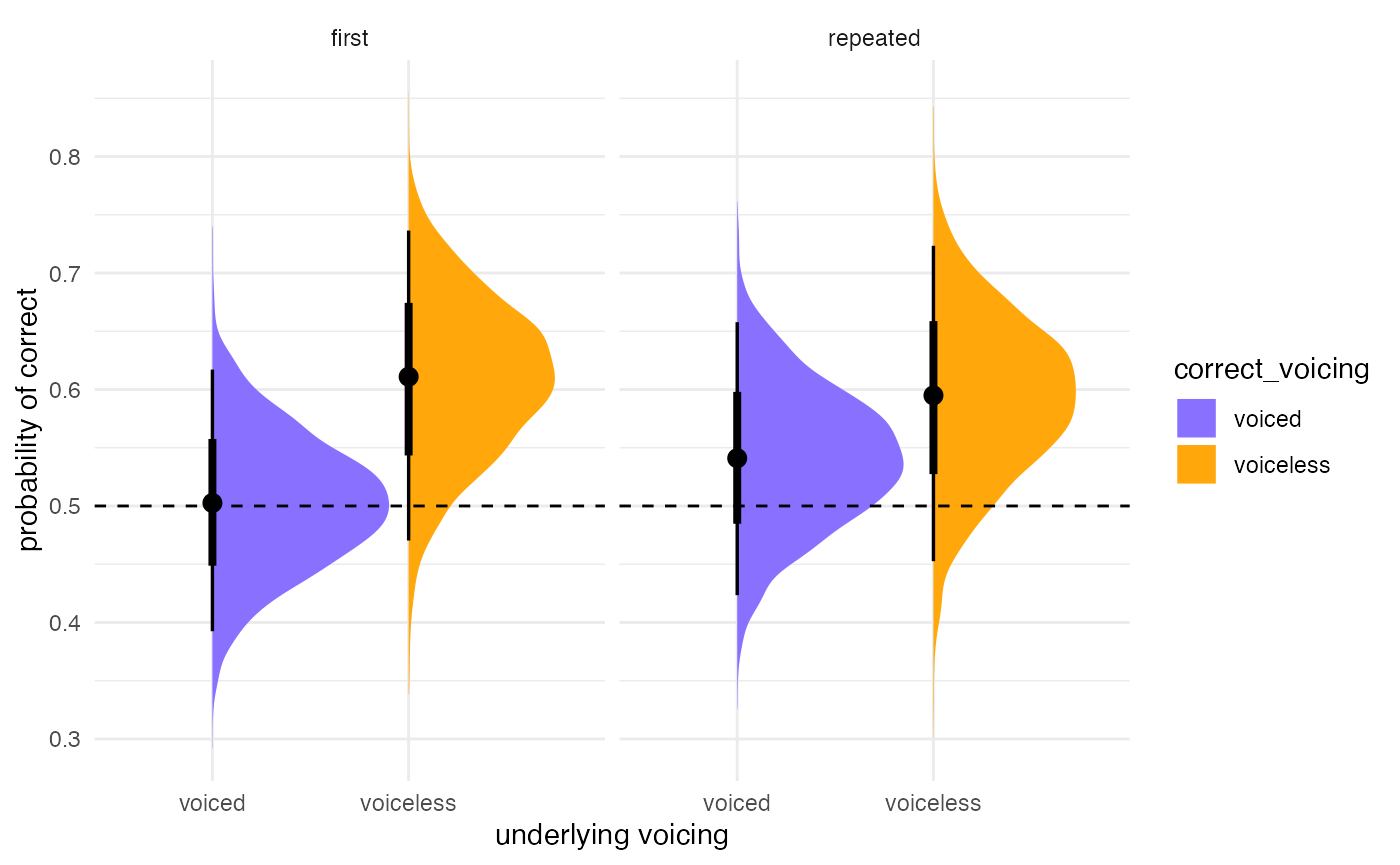

If you want to add the actual aggregated accuracy for each listener to the plot (for example), you can add that information on top. Makes for a very informative plot.

#aggregate
incomplete_agg <- incomplete %>% 
  group_by(listener, correct_voicing, repetitiontype) %>% 
  summarise(.value = mean(as.numeric(correct)), .groups = "drop")

post_plot +
  geom_point(data = incomplete_agg,
             aes(y = .value, 
                 x = correct_voicing, 
                 fill = correct_voicing),
             pch = 21, alpha = 0.5,
             position = position_nudge(x = -0.1))

Inference

Interpreting model output

# Describe posterior using fixef (to get simple, clean output... 
# focus on understanding each estimate in context and examining CrI's)
# Use in conjuction with levels_plot-2
fixef(m1_full)
#>                                                    Estimate  Est.Error
#> Intercept                                        0.01248959 0.23130872
#> correct_voicingvoiceless                         0.43899959 0.46065151
#> repetitiontyperepeated                           0.15628813 0.09375277
#> correct_voicingvoiceless:repetitiontyperepeated -0.22414533 0.13267918
#>                                                        Q2.5      Q97.5
#> Intercept                                       -0.43687340 0.47723123
#> correct_voicingvoiceless                        -0.45357875 1.33148511
#> repetitiontyperepeated                          -0.02722672 0.33584627
#> correct_voicingvoiceless:repetitiontyperepeated -0.48584540 0.03186847

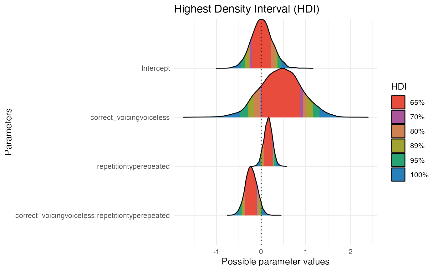
# Focus on describing posterior
hdi_range <- bayestestR::hdi(m1_full, ci = c(0.65, 0.70, 0.80, 0.89, 0.95))
hdi_range
#> Highest Density Interval
#> 
#> Parameter                                       |        65% HDI |        70% HDI |        80% HDI |        89% HDI |       95% HDI
#> -----------------------------------------------------------------------------------------------------------------------------------
#> (Intercept)                                     | [-0.21,  0.21] | [-0.25,  0.23] | [-0.27,  0.32] | [-0.36,  0.37] | [-0.46, 0.45]
#> correct_voicingvoiceless                        | [ 0.01,  0.87] | [-0.01,  0.93] | [-0.16,  1.02] | [-0.29,  1.16] | [-0.47, 1.31]
#> repetitiontyperepeated                          | [ 0.07,  0.25] | [ 0.07,  0.26] | [ 0.03,  0.27] | [ 0.00,  0.30] | [-0.03, 0.34]
#> correct_voicingvoiceless:repetitiontyperepeated | [-0.35, -0.11] | [-0.36, -0.09] | [-0.39, -0.05] | [-0.42,  0.00] | [-0.49, 0.03]

plot(hdi_range, show_intercept = T)